Machine Learning: An Introduction to Gradient Boosting

Welcome to the third article in our Machine Learning with Ruby opens a new window series!

In our previous article Machine Learning: An Introduction to CART Decision Trees in Ruby opens a new window , we covered CART decision trees and built a simple tree of our own. We then looked into our first ensemble model technique, Random Forests, in Machine Learning: An Introduction to Random Forests opens a new window . It is a good idea to review that article before diving into this one.

Random Forests are great for a wide variety of cases, but there are also situations where they don’t perform quite as well. In this article we’ll take a look at another popular tree-based ensemble model: Gradient Boosting.

Introduction

Ensemble models are a pretty powerful technique. Conceptually, they can be built with any kind of weak learner, and can handle both regression and classification (binary or multi-class) tasks.

A weak learner is a model that is only slightly better than random choice. Considering a binary classification problem, if you pick a class at random for a particular instance, you have a 50% chance of being right. Weak learners are only slightly better than that.

For the purposes of this article, we’ll focus on a specific type of weak learner: decision trees. It is important to note that decision trees are weak learners when shallow and, in ensemble models, trees are kept intentionally shallow. A standalone tree can be a strong learner if allowed to grow complex enough.

We’ll also focus on a specific type of problem, the one applicable to the use case described in our Machine Learning Aided Time Tracking Review: A Business Case article opens a new window , binary classification.

Brief Introduction to Gradient Boosting Classification

Gradient Boosting is a technique that builds a series of decision trees sequentially, with each individual tree designed to correct the errors made by previous trees. Instead of a “voting committee” approach like Random Forests, where predictions from individual trees are pooled and the most “voted” class is chosen, Gradient Boosting focuses on progressively reducing the residual errors of the model by using these residuals to train each new tree.

To make this easier to visualize, we can think of Gradient Boosting as a team of experts working towards an answer. Each new expert learns from the mistakes of the previous ones and gets a little bit closer to the answer. These “mistakes” are what’s called residuals.

The final prediction of the ensemble is then derived by combining the output of all the trees, effectively refining the accuracy of the model with each step. In other words, it iteratively enhances weak learners to build a robust and precise model that is effective in complex classification (and regression) tasks.

But why combine the output of all the trees to get a prediction if the last one is the most accurate?

Gradient Boosting is an additive process, meaning it relies on the “cumulative wisdom” of all these trees to work. The trees are sequential, they build upon the predictions of the previous trees, but don’t replace them. Each tree is trying to predict the residuals, not the actual target, so that the residuals get smaller with each tree, indicating the model is getting closer to the true target values. It’s a bit like a relay race, where each runner builds on top of the distance already run by the previous runner to get closer to the finish line. This also means the last tree is not fully informed, it only addresses the residuals that remain after all previous trees have made their contributions. For an actual target prediction, we need the cumulative contributions of all the trees.

Some important concepts to know when it comes to Gradient Boosting:

Boosting: Boosting is an ensemble technique that builds multiple weak learners sequentially, with each new tree correcting the errors of its predecessors. It constructs a decision tree, calculates the errors (distance between actual and predicted values) of the tree trained on the dataset, and then constructs a new tree focused on accurately predicting the errors of the first one. The predictions of the new tree are combined with the ones of the previous tree via a weighted sum, with more accurate trees being given more weight.

Loss Function: The loss function is the mathematical function that measures the difference between the values predicted by the model and the actual target values.

Gradient Descent: Optimization technique used to minimize the loss function by iteratively improving the model. The gradient in this context refers to the derivative (or rate of change) of the loss function with respect to the model’s predictions. Descent refers to the idea of moving in the opposite direction of the gradient to minimize said loss function. The gradient points towards the steepest increase in loss, so by moving in the opposite direction, we head towards reducing said loss (i.e. improving the model’s predictions). In Gradient Boosting, we often refer to fitting the trees to the “negative gradient”, which essentially means fitting the trees to the direction that will most reduce the loss, considering a negative gradient points to the direction of loss reduction, while the positive gradient would point towards increasing the loss.

Learning Rate: A regularization strategy that scales the contribution of each weak learner to control how fast the model learns. A lower rate means slower learning, while a higher rate means faster learning. It closely relates to the number of trees in the ensemble; lower learning rates will require a higher number of trees. However, it can lead to more robust models by not converging too quickly and helping avoid poor generalization and overfitting.

Odds: The ratio of the probability that an event will occur to the probability that it won’t. For an event with probability \(p\), it is defined as \(Odds = \frac{p}{1-p}\).

Log-Odds: The natural logarithm (logarithm to the base \(e\)) of the odds, defined as: \(LogOdds = ln(\frac{p}{1-p})\). Log-Odds are used in many implementations of Gradient Boosting for classification to make the initial prediction for each instance. The usage of log-odds helps transform the non-linear relationship between input features and the output into a more linear one, and provides a bounded range for the output, considering odds can range from 0 to infinity.

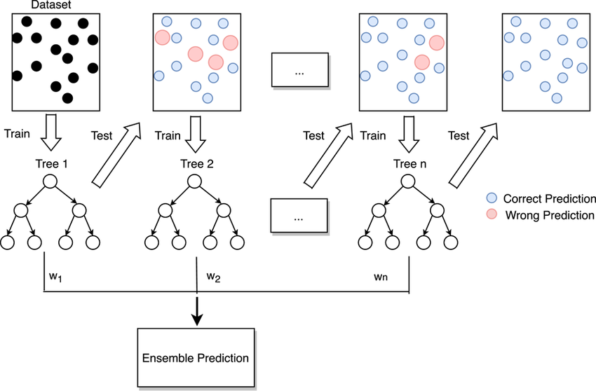
Representation of a Gradient Boosting classification process. Source: Improving Convection Trigger Functions in Deep Convective Parameterization Schemes Using Machine Learning by T. Zhang et al. (2021).

Gradient Boosting Classifier Algorithm

Gradient Boosting Classification works by sequentially building decision trees, with each new tree attempting to correct the errors made by its predecessors. Decision trees are built from the entire dataset, and the algorithm focuses on optimizing new trees by building them to correct the errors of the existing ensemble.

Before the first decision tree is built, an initial, very simple and naive prediction is made. The goal of the decision trees in Gradient Boosting is to minimize the loss function. Different loss functions are available, the default for Scikit-learn’s implementation being log-loss, which, for binary classification, is defined as

Where \(y\) is the actual label (for binary classification, 0 or 1), and \(p\) is the probability of the instance in question belonging to the positive class (represented by 1).

This initial prediction (initial set of residuals) will be the log-odds of the class probabilities, calculated from the class distribution of the training data supplied.

Note that these residuals are real numbers, not probabilities, and per the log-loss definition, we need the probability of an instance belonging to the positive class. To turn a residual into a probability, we use the sigmoid function, defined as

The sigmoid function maps any real-valued number into the 0 to 1 range.

Now, we can calculate pseudo-residuals from this initial prediction. These will be the derivative of the log-loss function with respect to the predicted probability \(p\):

In the context of Gradient Boosting, the term \(\frac{1}{p(1-p)}\) can be ignored, as it scales the gradient but does not change its direction. Therefore, the gradient used to update the model will effectively be \(y-p\).

This is the negative gradient of the loss function, and it guides how to adjust the prediction to reduce the loss. The gradient represents the changes needed to the log-odds (natural logarithm of the ratio of the probability of an event happening to the probability of it not happening) of the predictions for the model to improve its accuracy. A positive gradient means the model should increase the log-odds of the particular instance being in the positive class (1) while a negative gradient suggests that the model should decrease the log-odds. It is important to remember that in Gradient Boosting, the residual indicates how much change is needed in the log-odds (not directly in target probability) to reduce the loss.

So we take the first set of residuals, convert it to probabilities, and then for each one calculate the difference between the probability and the actual class (gradient of the log-loss function) to get the pseudo-residuals.

The first decision tree is then constructed on the training data. Unlike a standalone decision tree, instead of predicting the actual target label, it attempts to predict the gradient of the loss function relative to the model’s predictions. Essentially, for this initial tree, it tries to predict the errors or differences between its own predictions and the true values. Practically, this means that instead of feeding the tree the dataset and labels, we feed it the dataset and pseudo-residuals.

The goal of the first tree is to predict these residuals as accurately as possible. Once it’s trained, for each sample in the dataset, we get the prediction of the decision tree. This prediction is then multiplied by a learning rate (between 0 and 1). If we consider \(F_m(x_i)\) the prediction of the model for the \(ith\) instance of \(x\) after \(M\) boosting iterations, the scaling of the contribution of that tree is defined as:

Where \(v\) is the learning rate and \(h_m\) is the newly added tree.

The ensemble’s prediction is then updated with the prediction of the new tree, via weighted sum. Effectively, this means updating the first set of residuals with the first tree’s predictions for each sample, scaled by the learning rate.

The same process of converting the now updated residuals into probabilities using the sigmoid function and then calculating the pseudo-residuals is followed; and a second tree can be constructed to predict these pseudo-residuals, thus learning from the mistakes of the first tree. Similarly, once it’s trained, its own predictions will be scaled based on the learning rate and used to update the ensemble’s predictions.

The process of adding a new tree, calculating the pseudo-residuals, training the tree, scaling the tree’s predictions and updating the residuals of the ensemble is repeated until a specified maximum number of trees is reached or until adding more trees does not significantly decrease the loss function. The model then outputs its prediction, which is the weighted sum of predictions from all the trees in the ensemble up to that point. This total can be any number on the number line and can be represented as:

For classification tasks, we want a probability between 0 and 1, not any real number. Therefore, the result of the sum needs to be converted into a probability. To do so, we need to map the value of the prediction \(F_m(x_i)\) to a class or a probability, based on the loss function. The probability that a given instance of \(x\) belongs to the positive class (1) is:

where \(\sigma\) is the sigmoid function of \(F_m(x_i)\).

This transformation helps determine which class a prediction belongs to by using a decision threshold, typically 0.5 for binary classification.

Building a Gradient Boosting Classifier

Now that we have a good understanding of Gradient Boosting and gradient boosted trees, let’s leverage our DecisionTree class and build a very simple GradientBoostingClassifier of our own. The DecisionTree class here refers to an individual decision tree. For more information on decision trees and a simple sample implementation, check out our Machine Learning: An Introduction to CART Decision Trees in Ruby article opens a new window .

Like with the DecisionTree, we want a train method and a predict method. The difference is the train method of the classifier will call the DecisionTree’s train method on the pseudo-residuals of the original data.

First, we’ll initialize three things we’ll need: the maximum number of trees to construct, the learning rate we want, and the maximum depth we want for each individual tree in the ensemble. We’ll need to store the trees in an array and to store the prediction.

def initialize(max_tree_depth: 3, n_trees: 100, learning_rate: 0.1)
  @n_trees = n_trees
  @learning_rate = learning_rate
  @max_tree_depth = max_tree_depth
  @trees = []
  @initial_prediction = nil
end

Our train method will take in two variables: the data to train on and the target labels for the dataset. We first need to initialize the model and calculate the log-odds of the positive class, so we can calculate the first set of residuals:

positive_probability = labels.count(1).to_f / labels.size
@initial_prediction = Math.log(positive_probability / (1 - positive_probability))
residuals = Array.new(labels.size, @initial_prediction)

Now, for as many trees as specified, we’ll convert these log odds to probabilities, calculate a set of pseudo-residuals associated with them, and use these pseudo-residuals to train a new tree. Finally, for each new trained tree, we’ll update the total residuals (log odds) of the ensemble.

@n_trees.times do
  probabilities = residuals.map { |log_odds| 1.0 / (1.0 + Math.exp(-log_odds)) }

  pseudo_residuals = labels.zip(probabilities).map { |y, prob| y - prob }

  tree = DecisionTree.new
  tree.train(data, pseudo_residuals, max_tree_depth)
  @trees << tree

  data.each_with_index do |sample, index|
    tree_prediction = tree.predict(sample)
    residuals[index] += @learning_rate * tree_prediction
  end
end

That concludes our train method.

For the prediction, our predict method needs to, for each tree, gather its individual prediction and update the residuals (log odds) of the ensemble. It will then convert the final number to a probability and return the binary class prediction. Assuming a decision threshold of 0.5:

def predict(sample)
  log_odds = @initial_prediction
  @trees.each do |tree|
    prediction = tree.predict(sample, 0) # zero here is the default label to be used in case a standard prediction cannot be made for any reason
    log_odds += @learning_rate * prediction
  end

  probability = 1.0 / (1.0 + Math.exp(-log_odds))
  probability >= 0.5 ? 1 : 0
end

Putting it all together, we have a very simple Gradient Boosting Classifier:

require_relative "decision_tree"

class GradientBoostingClassifier
  attr_accessor :n_trees, :learning_rate, :max_tree_depth, :trees, :initial_prediction

  def initialize(max_tree_depth: 3, n_trees: 100, learning_rate: 0.1)
    @n_trees = n_trees
    @learning_rate = learning_rate
    @max_tree_depth = max_tree_depth
    @trees = []
    @initial_prediction = nil
  end
  
  def train
    positive_probability = labels.count(1).to_f / labels.size
    @initial_prediction = Math.log(positive_probability / (1 - positive_probability))
    residuals = Array.new(labels.size, @initial_prediction)

    @n_trees.times do
      probabilities = residuals.map { |log_odds| 1.0 / (1.0 + Math.exp(-log_odds)) }

      pseudo_residuals = labels.zip(probabilities).map { |y, prob| y - prob }

      tree = DecisionTree.new
      tree.train(data, pseudo_residuals, max_tree_depth)
      @trees << tree

      data.each_with_index do |sample, index|
        tree_prediction = tree.predict(sample)
        residuals[index] += @learning_rate * tree_prediction
      end
    end
  end

  def predict(sample)
    log_odds = @initial_prediction
    @trees.each do |tree|
      prediction = tree.predict(sample, 0)
      log_odds += @learning_rate * prediction
    end

    probability = 1.0 / (1.0 + Math.exp(-log_odds))
    probability >= 0.5 ? 1 : 0
  end
end

We’re all set! We now have a very simple Gradient Boosting Classifier of our own. Like with Random Forest, for actual use cases, we need a much more robust algorithm which is, again, why we used Scikit-learn to build our own. The goal of this demonstration is to explain the basic concepts behind how this kind of classification works.

For more information on Scikit-learn’s implementation of Gradient Boosting Classifiers and how to use them, check out their documentation opens a new window .

Conclusion

First, we built our very own decision tree. Now we have built two different kinds of ensemble models: Random Forests and Gradient Boosting classifiers. As you can image, though, Gradient Boosting can be quite slow, as all trees are built sequentially. Next in this series we’ll take a look at more advanced implementations of the Gradient Boosting algorithm: XGBoost (eXtreme Gradient Boosting) and LightGBM (Light Gradient Boosting Machine). These implementations offer improved speed, performance and some additional features compared to traditional Gradient Boosting methods.

Excited to explore the world of Machine Learning opens a new window and how it can be integrated into your application? We’re passionate about building interesting, valuable products for companies just like yours! Send us a message over at OmbuLabs! opens a new window